How Animal Movements Help Us Study the Planet

Scientists have been underutilizing a key resource we can use to help us understand Earth: animals. Our fellow Earthlings have a much different, and usually much more direct, relationship with the Earth. They move around the planet in ways and to places we don’t.

What can their movements tell us?

Humanity has a fleet of satellites orbiting Earth that tell us all kinds of things about the planet. Satellites track temperature, CO₂ emissions, rainfall, forest fires, drought, volcanic eruptions, etc. We know more about Earth than ever, and a lot of it is thanks to satellites.

Climate change is our biggest concern right now, and new research shows that sensors attached to animals can elevate our climate change data to a new, more granular level.

The research perspective is titled “Animal-borne sensors as a biologically informed lens on a changing climate,” published in Nature Climate Change. The lead author is Diego Ellis-Soto, a graduate student at Yale University and a NASA FINESST (Future Investigators in NASA Earth and Space Science and Technology) fellow.

The first animal tracker was probably just a piece of coloured string. In 1803, American Naturalist John Audobon wanted to know if birds migrated and returned to the same place yearly. So he attached a piece of string around a bird’s leg before it flew south for the winter. Next spring, he spotted the bird and knew it had returned to the same place.

The tools at scientists’ disposal now are much more powerful than Audobon’s piece of string. Ellis-Soto studies animal movements and what they can tell us about rapid environmental change. He uses remote sensing, GPS tracking, and citizen science to try to forecast environmental changes at fine spatio-temporal scales.

This type of research has its roots in things like the Great Backyard Bird Count, where citizen scientists spend four days each February recording what birds they see. Participants spend only a few minutes each day recording what they see and uploading it to a website. The result is a massive collection of data unattainable by any other method.

The Bird Count is a more passive example of animal movement studies that the authors advocate. They’re pursuing more active methods of studying animal movement and gathering data to get around some of the roadblocks scientists face when studying the climate.

“Traditional climate measurements are often constrained by geographically static, coarse, sparse and biased sampling, and only indirect links to ecological responses,” Ellis-Soto and his co-authors write in their research. “Here we discuss how animal-borne sensors can deliver spatially fine-grain, biologically fine-tuned, relevant sampling of climatic conditions in support of ecological and climatic forecasting.”

A 130-pound wolf watches biologists in Yellowstone National Park after being captured and fitted with a radio collar on 1-9-03. Tracking wolves as they move through their territory can also tell researchers about the environmental and climate conditions that motivate their movements. Image Credit: By William C. Campbell – U.S. Fish & Wildlife Service, Public Domain, https://ift.tt/aB7ENpY

Even though we have a fleet of powerful satellites and a massive number of ground-based data collectors, they each have a weakness of some type. Ground stations can only sample data from a single location. Satellites have their own limitations. They can collect data in fine spatial resolution, across multiple wavelengths, or at high temporal frequency. But they don’t do it all at once. They’re also inhibited by cloud cover and, in some cases, the darkness of night. The result is data that though powerful, has gaps in it.

Animal sensors can bridge those gaps, according to Ellis-Soto. “Animals are an integral component of Earth observation,” he said.

Animal-borne sensors (ABS) aren’t new. They’ve been used for decades to track various animals, including predators like lions, ocean-going animals like orcas, migrating birds, and even insects. These trackers monitor and report an animal’s movements in places that satellites can’t monitor, and humans can’t easily access. But Ellis-Soto says we can use trackers to gather other data, like temperature.

In South Africa’s Kruger National Park, scientists used temperature and movement trackers on elephants to monitor the animals as they moved around in the park for one year. They combined it with satellite temperature data. Two maps from that effort show how the elephant sensors filled in gaps in the satellite data and created a much more complete picture.

These two maps show satellite temperature data (top) and elephant location and temperature data from ABSs. Image Credit: NASA Earth Observatory images by Michala Garrison, using Landsat data from the U.S. Geological Survey and elephant-borne sensor data from Thaker, M. et al. (2019).

Ellis-Soto sees the issue in terms of bias. Each satellite has a sampling bias. Sampling bias is unavoidable when designing satellites and their instruments. But animals have a sampling bias, too, and scientists can use that bias for their own purposes.

“These animals are extremely biased sensors, and this bias is called animal ecology and behaviour,” said Ellis-Soto.

The elephants in Kruger National Park are just one example. The use of ABSs is widespread.

This image shows how ABSs are used to collect different environmental data. 1 to 9 show ABSs used to estimate measurements ranging from wind speed and direction to air temperature. 10 to 16 shows ABSs used to measure sea surface temperature and salinity. 17 and 18 show ABSs used to measure near-surface temperature in terrestrial realms. Image Credit: Ellis-Soto et al. 2023

Ellis-Soto and his colleagues see many opportunities to expand this kind of monitoring and combine it with other data, including satellite data. “Technological advances in ABSs offer an ever-increasing number and quality of auxiliary on-board sensors that collect climatic variables,” they write. Technological advancements in ABSs combined with animal movement are powerful tools that can play a larger role. “Animals can access and monitor remote areas and detect rare events and hard-to-measure environmental conditions of potential importance for climate change projections.”

The authors highlight the issue of snowmelt. Around the world, snowmelt is an important indicator in understanding the coming growing season. Snowmelt provides irrigation water for millions of farmers around the world. For example, in India and Pakistan, 130 million farmers rely on meltwater to irrigate their crops.

“In many areas of the globe, snowmelt is a crucial component of the natural hydrological cycle,” they write. “A biological warning system of earlier snowmelt under climate change by ABSs may improve estimates of the contribution to mountain hydrology, a critical area of improvement for climate change projections and water runoffs for food production.”

In the Arctic, researchers used ABSs to track the movements of three types of birds: snowy owls, rough-legged buzzards, and peregrine falcons. The ABS data showed how these animals follow the snowmelt during migratory journeys. The data was more granular than satellites could provide. “Spatially fine-scaled capture of patches of snowmelt as homed in on by animals is otherwise hard to attain but highly useful for understanding the phenology and distribution of Arctic species under changing climate conditions,” the authors write.

There are many examples of ABSs being used to gather otherwise unattainable or difficult-to-obtain environmental data. But there are also many more opportunities waiting to be realized.

This figure shows how harp seals can be fitted with ABSs to record and transmit data while going about their business. ARGOS is a satellite network dedicated to wildlife monitoring. Image Credit: McMahon et al. 2021.

“We see a real opportunity for the ecological and meteorological community to employ ABSs for a strongly expanded, representative and biologically interpretable measurement of meteorological
and climatic conditions under current and future climate,” the authors write.

Our fellow Earthlings are like an army of unwitting citizen scientists. As long as the ABSs don’t hamper or harm them, they can greatly contribute to Earth’s well-being without even knowing it.

“The thousands of animals today swimming, running and flying around the globe carrying electronic tags are agile earth observers with the potential to provide transformative data collection in support of global change research, meteorology, climate forecasting and ecology,” the authors conclude.

The post How Animal Movements Help Us Study the Planet appeared first on Universe Today.

Mapping Lava Tubes on the Moon and Mars from Space

Sometimes, all you need for a new discovery is some creative math. That was the case for a new paper by Edward Williams and Laurent Montési of the University of Maryland’s Department of Geology. They released a brief paper at the Lunar and Planetary Science Conference last month that describes a mathematical way to estimate the size of a lava tube using only remote sensing techniques.

A critical starting point was the discovery that the ridge height of a surface above a lava tube is proportional to the cube of the height of the lava tube’s roof. Plenty of lava tubes have been studied in detail on Earth, and those studies were used to form the basis of that equation.

However, until now, there was no relationship between the roof thickness and the details of the shape of the lava tunnel itself. Enter physical modeling – the authors used a physics modeling program (COMSOL Multiphysics) to model different roof heights based on different characteristics of tunnels.

Fraser looks at how we might explore laval tubes.

One big difference was the form of the tunnel itself – they focused on two styles. One, known as “laccolith,” was a rectangle, whereas most people would think of a half-ellipse style when considering lava tubes. The modeling program also had to consider things like the material strength of the regolith as well as the pressure inside the tunnel itself – which would usually match the outside atmospheric pressure of largely airless worlds like the Moon and Mars, assuming there is a hole that connects it to the greater atmosphere.

The equation the authors eventually found uses some fancy calculus and is beyond the scope of this article. Still, their model seems to fit the data for most modeled lava caves, including those on Earth.

They turned their model to a well-known cave structure on Earth to prove that point. Valentine’s Cave, located in the Lava Beds National Monument in California, has been studied for decades by NASA researchers as an analog to caves found on the Moon and Mars. Those studies have resulted in accurate cave heights and ridge height estimates using techniques such as LIDAR.

When applying their new model and using the known ridge height of Valentine’s Cave, the authors find a tube height within .07 m of the actual height of the Cave. Not bad for calculating the height only from the ridge height, which is an externally visible feature.

Lava tubes are a central feature of any future crewed exploration mission.

The obvious next step is to attempt to estimate some lava tube heights on our neighboring planetary bodies. At least some remote observatories around the Moon and Mars should be capable of estimating ridge height from their orbital positions. It’s then up to the team to estimate what the inside of the tube might look like. Unfortunately, it will probably be a while before human or robotic explorers enter one of these tubes to confirm the author’s estimates. But there are plenty of proposals for that as well – and one day, undoubtedly, someone or something will indeed step foot inside one of these ancient geological formations.

Learn More:
William & Montési – DETERMINATION OF LAVA TUBE DEPTH AND SHAPE FROM TOPOGRAPHY
UT – It’s Time to Study Lunar Lava Tubes. Here’s a Mission That Could Help
UT – Future Mars Helicopters Could Explore Lava Tubes
UT – Lava Tubes on the Moon Maintain Comfortable Room Temperatures Inside

Lead Image:
Lava tube on Mars
Credit – NASA/JPL-Caltech/University of Arizona

The post Mapping Lava Tubes on the Moon and Mars from Space appeared first on Universe Today.

A Robot Hopper to Explore the Moon’s Dangerous Terrain

Intuitive Machines recently had a major breakthrough, successfully becoming the first non-governmental entity to land on the Moon in February. At least the landing was partially successful – the company’s Odysseus lander ended up on its side, though its instruments and communication links remained at least partially functional. That mission, dubbed IM-1, was the first in a series of ambitious missions the company has planned. And they recently released a paper detailing features of a unique hopping robot that will hitch a ride on its next Moon mission.

Known as South Pole Hopper (or S.P. Hopper), the robot will be the first of a new class called µNova. Weighing in at only 35 kg and standing only 70 cm tall, this miniaturized craft is a stand-alone spacecraft that can operate entirely autonomously. It must do this to complete its mission of exploring the region around the permanently shadowed regions (PSRs) at the lunar south pole.

Specifically, the craft has four distinct objectives: 

1. Determine the geologic properties of a specific ridge at the south pole, including inside a PSR
2. Determine the surface brightness temperatures of both areas bathed at least partially in the Sun’s rays and also in the PSR.
3. Research the “surface roughness” and “thermal inertia” of the Moon’s regolith at its landing location.
4. Determine how much hydrogen there is in the general area – with the understanding that, most likely, it will be tied up in water.

Video about the IM-2 Mission
Credit – NASASpaceNews

None of those objectives individually require S.P. Hopper’s most notable feature – but it sure would be helpful to complete them – it can “hop” by thrusting itself off the lunar surface and landing in an area it chooses completely autonomously – even in a PSR. It can do so at an angle of up to 10 degrees, the company is quick to point out, given its recent difficulties with spacecraft angle. 

The paper describes several technical features of the hopper – including the fact that it will use a wireless LTE system to communicate. To collect the data required for its mission, it has three main scientific instruments: a set of CMOS cameras, whose primary task is to help with autonomous navigation but can also send pictures back to Earth to be analyzed; the LRAD thermopile sensor system; designed to capture brightness measurements of the regolith, and the PLWS, a miniature neutron spectrometer, specifically designed to look for hydrogen in space.

However, perhaps the most interesting part of the paper details its flight plan. S. P. Hopper is designed to make 5 – possibly 6 – hops when it lands at the lunar south pole. The first will be a “commissioning hop” that will only traverse 20 m or so. Next will be a 100 m “proof of concept” hop that will demonstrate that a hopping robot is a viable mode of transportation on the Moon.

Following those initial flights, S. P. Hopper will fly about 300 m to the rim of Marston crater, part of the Shackleton – de Gerlache ridge. It will then fly into the crater itself, which is a PSR, and then fly back out to the ridge again. If there’s enough fuel left, Intuitive Machines plans a 6th exploratory flight to look at anything interesting in the vicinity. 

Fraser discusses Intuitive Machine’s lunar landing.

Currently, IM-2, the flight that will take S.P. Hopper to the South Pole, is scheduled for launch sometime this year. Given Intuitive Machine’s relative success with the Odysseus lander, there’s a lot of optimism about the success of this mission as well. For now, though, we’ll have to wait and see if the company can pull off an even more successful follow-on mission.

Learn More:
Martin et al – S.P. HOPPER: IN-SITU EXPLORATION OF THE SHACKLETON DE GERLACHE RIDGE
UT – NASA is Going Ahead With a Hopping Lander to Explore the Lunar Surface
UT – China’s Chang’e-7 Will Deploy a Hopper that Jumps into a Crater in Search of Water Ice
UT – Drones Could Help Map the Lunar Surface with Extreme Precision

Lead Image:
View of the S.P Hopper.
Credit – Martin et al.

The post A Robot Hopper to Explore the Moon’s Dangerous Terrain appeared first on Universe Today.

Inside a Week to Totality: Weather Prospects, Solar Activity and More

Looking at prospects for eclipse day and totality.

Have you picked out your site to observe the eclipse on April 8^th? Next Monday, the shadow of the Moon crosses Mexico, the contiguous United States from Texas to Maine, and the Canadian Maritimes for the last time for this generation. And while over 30 million people live in the path of totality, millions more live within an easy day drive of the path. I’m expecting that many folks will decide to make a three-day weekend of it, and eclipse travel traffic will really pick up this coming Saturday, April 6^th.

We’ve written previously on observing and safety in our big guide to the April 8^th total solar eclipse, and the science campaigns underway to meet the eclipse.

So, what can we expect on the big day? While eclipses and celestial mechanics are a definite, not all eclipses are the same, as key variables both cosmic and terrestrial play a role in the experience.

Watching the Weather

Of course, the major question mark that everyone is watching is weather and cloud cover. As the day nears, weather models begin to merge and agree. While climate models typically favor clear skies in early April for the southwest portion of the track and clouds to the northeast, predictions now actually show a reverse trend for the afternoon of the 8^th. This means clear skies for New England, and clouds (and perhaps, even afternoon storm and tornado warnings) to the south towards Texas. Keep in mind, a Nor’easter is also inbound for New England late this week… we actually opted to head to northern Maine early for this very reason. Good sites to check include Pivotal Weather, and NOAA’s cloud cover forecast. On eclipse day, we’re watching the GOES-East live view page on North America to see what’s actually occurring.

Cloud cover prospects of April 8th, versus the eclipse path. Credit: Pivotal Weather.

It’s always tough to know if the Sun will be obscured by a cloud for the scant few minutes of totality days prior. Remember: you don’t need a pristine clear sky for a solar eclipse… just a good view of the Sun and Moon. April over North America can be a fickle month.

Sometimes, seeing the eclipsed Sun through thick fast-moving clouds can provide a memorable view. This was the case for us in 2017 when we caught the eclipse from PARI, North Carolina in the Smoky Mountains.

Solar Activity

We’re now headed towards the peak of Solar Cycle No. 25, so expect the Sun to be active, come eclipse day. Sunspots rotating into view now will also be visible during the partial phases of the eclipse leading up to totality. The Sun is uncharacteristically quiet this week, but we do have a few sunspots rotating into view to add a photogenic look to the Sun.

Sunspot activity rotating into view as of April 3rd. NASA/ESA/SOHO

The Corona’s Appearance

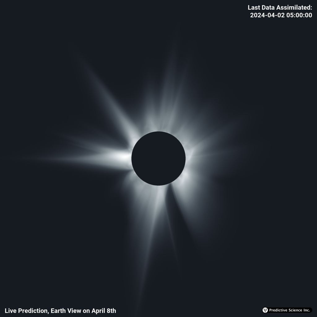
Did you know: long-time eclipse chasers can actually identify which eclipse a given photo is from… just from the appearance of the corona. Predictive Science Incorporated actually runs a forecast for the appearance of the corona come eclipse day, and it looks like we’re in for a memorable one:

The latest prediction for the appearance of the solar corona on eclipse day. Credit: Predictive Science Inc.

Catching the International Space Station transiting the partially eclipsed Sun can be a memorable observation. ISS Transit Finder is a good site to predict transits of the station for a given location.

A transit of the ISS captured during the 2015 partial solar eclipse. Credit: Thierry Legault.

Last Minute Plans

Mobility is key, come eclipse day. Plan your eclipse expedition like a heist, complete with a plan to go mobile and an escape route. Tales of totality are replete with stories of eclipse chasers driving down back roads and even taking off running on foot to stay ahead of incoming clouds.

Skywatching During Totality

Though totality is fleeting, do take about half a minute to stargaze. Jupiter and Venus will be visible, along with several +1^st magnitude stars. Comet 12P Pons-Brooks is also at +4.5 magnitude in the constellation Aries, 25 degrees from the Sun. A well-placed outburst from this tempestuous comet could always vault it into binocular or even naked eye visibility.

Skywatching during totality. Credit: Stellarium.

Animal Activity During Totality

Finally, keep an eye (and ear) out for any anomalous phenomena during totality. Temperatures may drop, roosters may crow, and nocturnal creatures may briefly emerge, fooled by the false twilight. In 2017, we faced a sudden onslaught of mosquitoes as midday darkness descended.

If you have the means, do make sure you’re in the path of totality come eclipse day. This one has a special significance for us, as it’s the only total solar eclipse that passes over our hometown of Mapleton, Maine in our lifetimes.

Good luck, safe travels to totality, and clear skies!

The post Inside a Week to Totality: Weather Prospects, Solar Activity and More appeared first on Universe Today.

Want to Leave the Solar System? Here’s a Route to Take

The edge of the Solar System is defined by the heliosphere and its heliopause. The heliopause marks the region where the interstellar medium stops the outgoing solar wind. But only two spacecraft, Voyager 1 and Voyager 2, have ever travelled to the heliopause. As a result, scientists are uncertain about the heliopause’s extent and its other properties.

Some scientists are keen to learn more about this region and are developing a mission concept to explore it.

The heliosphere plays a critical role in the Solar System. The Sun’s heliosphere is a shield against incoming galactic cosmic radiation, like that from powerful supernovae. The heliopause marks the extent of the heliosphere’s protective power. Beyond it, galactic cosmic radiation is unimpeded.

“We want to know how the heliosphere protects astronauts and life in general from harmful galactic radiation, but that is difficult to do when we still don’t even know the shape of our shield.”

Marc Kornbleuth, Boston University

There’s no overall understanding of the shape and extent of the heliosphere and heliopause. A new study wants to address that by designing a probe that would travel beyond this region to find the necessary answers.

The study is “Complementary Interstellar Detections from the Heliotail,” published in Frontiers in Astronomy and Space Sciences. The lead author is Sarah Spitzer, a postdoctoral research fellow in the Department of Climate and Space Sciences and Engineering at the University of Michigan.

“Without such a mission, we are like goldfish trying to understand the fishbowl from the inside,” said Spitzer.

The heliopause protects everything inside it from galactic cosmic radiation, including our astronauts who leave the Earth’s protective magnetosphere. “We want to know how the heliosphere protects astronauts and life in general from harmful galactic radiation, but that is difficult to do when we still don’t even know the shape of our shield,” said Marc Kornbleuth, a research scientist at Boston University and co-author of the study.

According to simulations, this image shows three models of what the heliosphere could look like. Left: a comet-like shape. Middle: The Croissant model. Right: A different, more streamlined comet-like shape. Image Credits are listed in the image.

The heliosphere’s shape comes from the interaction between the Sun’s solar wind and the local interstellar medium (LISM.) The LISM is made of plasma, dust, and neutral particles. Two clouds in the LISM dominate our region of space: the Local Interstellar Cloud and the G-Cloud, home of the Alpha Centauri system. Two other clouds, the AQL Cloud and the Blue Cloud, are nearby. The clouds are regions where the LISM is denser.

The problem scientists face is that we can’t learn much more about the heliosphere’s shape and its relation to the LISM and its clouds without getting outside the heliosphere. While Voyager 1 and 2 have wildly exceeded the most feverish expectations by lasting this long and leaving the heliosphere, they’re near the end. Their instruments don’t function as they used to, and even then, those spacecraft were built in the 1970s. It goes without saying that technology has advanced since then.

What we need is a purpose-built spacecraft that can leave the heliosphere when and where we want it to. Of course, that’s an extremely long journey, and it would fulfill other scientific objectives along the way. But unlike the Voyager probes, which were sent to study the planets and only reached the LISM through sheer stubbornness, this probe would primarily be designed to explore the heliopause.

This illustration shows the position of NASA’s Voyager 1 and Voyager 2 probes outside of the heliosphere, a protective bubble created by the Sun that extends well past the orbit of Pluto. Voyager 1 exited the heliosphere in August 2012. Voyager 2 exited at a different location in November 2018. Credit: NASA/JPL-Caltech

“A future interstellar probe mission will be our first opportunity to really see our heliosphere, our home, from the outside, and to better understand its place in the local interstellar medium,” said lead author Spitzer.

The idea has been around for a while. In 2021, scientists developed a mission concept for such a probe. They called it the Interstellar Probe and said it would embark on a 50-year-long journey into the LISM. They said it would “… provide the first real vantage point of our life-bearing system from the outside.” It could launch in 2036 and travel at a peak speed of 7 AU per year. That’s about one billion km per year.

The cover page from the 2021 proposal for a mission to leave the heliosphere. Image Credit: Interstellar Probe/JHUAPL

The exit point is a critical difference between the 2021 proposal and this one. The 2021 proposal stated that the probe should “Capture a side view of the heliopause to characterize shape, preferably near 45° off of the heliopause nose direction at (7°N, 252°E) in Earth ecliptic coordinates.”

The authors of this new paper say that the Interstellar Probe team got the exit point wrong. “However, this report assumes that a probe trajectory near 45 degrees off the nose of the heliotail, or the front of the Sun’s directional motion, is optimal,” they write. Spitzer and her colleagues examined the issue and came to a different conclusion. They investigated six different trajectories for a probe, from noseward to tailward. They concluded that a side view is best.

“If you want to find out how far back your house extends, walking out the front door and taking a picture from the front sidewalk is likely not your best option. The best way is to go out the side door so you can see how long it is from front to back,” said co-author Kornbleuth. This vantage point will give the best scientific results and view of the heliosphere’s shape.

“Understanding the shape of the heliosphere requires an understanding of the heliotail, as the shape is highly dependent upon the heliotail and its LISM interactions,” the authors write in their paper. “The Interstellar Probe mission is an ideal opportunity for measurement either along a trajectory passing through the heliotail, via the flank…”

There’s another compelling reason to follow this trajectory. Researchers think that plasma from the LISM might enter the heliosphere through its tail because of magnetic reconnection. If that’s true, the probe could sample the LISM twice: once inside the heliosphere and once outside of it.

The team also proposed that two probes be sent beyond the heliosphere. One would have a noseward trajectory, and the other would have a heliotailward trajectory. That would “… yield a more complete picture of the shape of the heliosphere and to help us better understand its interactions with the LISM,” they explain in their paper.

Recent research suggests that the Solar System is on a path that will take it out of the Local Interstellar Cloud (LIC.) It may already be in contact with four different clouds with different properties. Image Credit: Interstellar Probe/JHUAPL

“This analysis took a lot of persistence. It started small and grew into a great resource for the community,” said study co-author Susan Lepri.

The team behind the proposal says the Interstellar Probe will be a 50-year mission travelling 400 astronomical units. It could potentially travel much further, up to 1,000 astronomical units. According to the researchers, this would give us an unprecedented view of the heliosphere and the LISM.

The post Want to Leave the Solar System? Here’s a Route to Take appeared first on Universe Today.

Curiosity has Reached an Ancient Debris Channel That Could Have Been Formed by Water

Like a pilgrim seeking wisdom, NASA’s MSL Curiosity has been working its way up Mt. Sharp, the dominant central feature in Gale Crater. Now, almost 12 years into its mission, the capable rover has reached an interesting feature that could tell them more about Mars and its watery history. It’s called the Gediz Vallis channel.

Gediz Vallis channel appears to have been carved by ancient water. But if that’s the case, it happened billions of years ago. The channel has since filled with rock.

Mt. Sharp’s upper regions are beyond Curiosity’s reach. It’s simply too difficult for the rover to get there. But Nature is playing nice with MSL Curiosity. Rocks have come tumbling down from the mountain, creating a ridge and filling up a channel. Those rocks are within reach, and they could hold clues to Mars’ watery past.

Mars’ ancient history, especially as it concerns surface liquid water, is a gigantic puzzle with lots of pieces. We know there are hydrated minerals on Mars that date back millions of years. We know there are sulphates, which are minerals left behind when water evaporates. We have orbiter images clearly showing river channels and deltas.

Gediz Vallis is a tiny part of Mars, but it could make an important contribution to our understanding of this once warm and wet world.

This image from 2019 shows a proposed route for MSL Curiosity. The rover is about to expire Gediz Vallis Channel. Image Credit: By NASA/JPL-Caltech/ESA/Univ. of Arizona/JHUAPL/MSSS/USGS Astrogeology Science Center – https://ift.tt/G8hWiBy, Public Domain, https://ift.tt/7VRA5EC

Understanding Gediz Vallis and what it could tell us begins with Mt. Sharp. Mt. Sharp was built up over long periods of geological time by the deposit of sediments into layers. Over time, some of this material was eroded away, presenting us with what we see today. The Gediz Vallis channel formed after all that had happened.

Because the channel has steep walls, scientists say water had to carve it. Wind erosion is ruled out because it creates shallow, wide walls. Sometime after it formed, it was filled with rocky debris. That debris probably came from high up Mt. Sharp, beyond Curiosity’s reach. The rock will give the rover a look at the upper reaches of the mountain that it would otherwise never obtain.

This image shows the debris piles in the Gediz Vallis channel, as seen by MSL Curiosity. Image Credit: NASA/JPL-Caltech/UC Berkeley

Ashwin Vasavada is the Project scientist for NASA’s Curiosity rover at JPL. “If the channel or the debris pile were formed by liquid water, that’s really interesting,” he said in a press release. “It would mean that fairly late in the story of Mount Sharp – after a long dry period – water came back, and in a big way.”

This agrees with other evidence Curiosity found. Instead of disappearing once and for all, water seems to have come and gone in phases, confounding our attempts to understand Mars’ history.

Gediz Vallis Ridge is the hill-like slope at right in this MSL Curiosity image captured on August 19th, 2023. It took the rover three attempts over three years before it could reach the ridge. It spent 11 days at the ridge and is now working its way to Gediz Vallis Channel. The formation has scientists intrigued because of what it might tell them about the history of water on the Red Planet. Image Credit: NASA/JPL-Caltech

A year ago, the rover ascended the Gediz Vallis ridge, a sprawling debris pile that appears to grow out of the end of the channel, to get a closer look. Since the debris looks like it flows out of the channel, it indicates that both are results of the same geological process.

Even though MSL Curiosity is an engineering marvel, the rover will still need months to study the Gediz Vallis Channel. What it uncovers over the following months could give scientists a lot more detail about the history of Mars’ water.

Recently published research based partly on Curiosity’s data also shows that Mars had episodes of water and that it didn’t all disappear at once. That research showed that the bulk of Mt. Sharp was formed by waterborne sediments and that after that happened, another layer made of windborne sediments formed on top of it. But images of the windborne layer show that the sedimentary rock is deformed by the later presence of water.

This digital elevation model (DEM) provides some context for Curiosity’s journey. Image Credit: Hughes et al. 2022

How Gediz Vallis fits into Mars’ story is unclear. But getting a closer look will start to untangle the planet’s complex history. Was the channel carved by water? If Curiosity can confirm that, then it’s more evidence that Mars had surface water more recently than though. Did water carry the boulders and debris that filled it, or did dry avalanches?

Curiosity needs months to explore the region. Once researchers have had time to digest and interpret the rover’s data, we’ll get more answers.

The post Curiosity has Reached an Ancient Debris Channel That Could Have Been Formed by Water appeared first on Universe Today.

Where Are All These Rogue Planets Coming From?

There’s a population of planets that drifts through space untethered to any stars. They’re called rogue planets or free-floating planets (FFPs.) Some FFPs form as loners, never having enjoyed the company of a star. But most are ejected from solar systems somehow, and there are different ways that can happen.

One researcher set out to try to understand the FFP population and how they came to be.

FFPs are also called isolated planetary-mass objects (iPMOs) in scientific literature, but regardless of what name’s being used, they’re the same thing. These planets wander through interstellar space on their own, divorced from any relationship with stars or other planets.

FFPs are mysterious because they’re extremely difficult to detect. But astronomers are getting better at it and are getting better tools for the task. In 2021, astronomers made a determined effort to detect them in Upper Scorpius and Ophiuchus and detected 70 of them, possibly many more.

This image shows the locations of 115 potential rogue planets, highlighted with red circles, recently discovered in 2021 by a team of astronomers in a region of the sky occupied by Upper Scorpius and Ophiucus. The exact number of rogue planets found by the team is between 70 and 170, depending on the age assumed for the study region. This image was created assuming an intermediate age, resulting in a number of planet candidates in between the two extremes of the study. Image Credit: ESO/N. Risinger (skysurvey.org)

In broad terms there are two ways FFPs can form. They can form like most planets do, in protoplanetary disks around young stars. These planets form by accretion of dust and gas. Or they can form like stars do by collapsing in a cloud of gas and dust unrelated to a star.

For planets that form around stars and are eventually kicked out, there are different ejection mechanisms. They can be ejected by interactions with their stars in a binary star system, they can be ejected by a stellar flyby, or they can be ejected by planet-planet scattering.

In an effort to understand the FFP population better, one researcher examined ejected FFPs. He simulated rogue planets that result from planet-planet interactions and those that come from binary star systems, where interactions with their binary stars eject them. Could there be a way to tell them apart and better understand how these objects come to be?

A new paper titled “On the properties of free-floating planets originating in circumbinary planetary systems” tackled the problem. The author is Gavin Coleman from the Department of Physics and Astronomy at Queen Mary University of London. The paper will be published in the Monthly Notices of the Royal Astronomical Society.

In his paper, Coleman points out that researchers have explored how FFPs form, but there’s more to do. “Numerous works have explored mechanisms to form such objects but have not yet provided predictions on their distributions that could differentiate between formation mechanisms,” he writes.

Coleman focuses on ejected stars rather than stars that formed as rogues. He avoids rogue planets that are a result of interactions with other planets because planet-planet scattering is not as significant as other types of ejections. “It is worth noting that planet-planet scattering around single stars cannot explain the large number of FFPs seen in observations,” Coleman explains.

This artist’s impression shows an example of a rogue planet with the Rho Ophiuchi cloud complex visible in the background. Rogue planets have masses comparable to those of the planets in our Solar System but do not orbit a star, instead roaming freely on their own. Image Credit: ESO/M. Kornmesser/S. Guisard

Coleman singles out binary star systems and their circumbinary planets in his work. Previous research shows that planets are naturally ejected from circumbinary systems. In his research, Coleman simulated binary star systems and how planets ejected from these systems behave. “We find significant differences between planets ejected through planet-planet interactions and those by the binary stars,” he writes.

Coleman based his simulations on a binary star system named TOI 1338. TOI 1338 has a known circumbinary planet called BEBOP-1. Using a known binary system with a confirmed circumbinary planet provides a solid basis for his simulations. It also allowed him to compare his results with other simulations based on BEBOP-1.

The simulation varied several parameters: the initial disc mass, the binary separation, the strength of the external environment, and the turbulence level in the disc. Those parameters strongly govern the planets that form. Other parameters used only a single value: the combined stellar mass, mass ratio and binary eccentricity. The combined stellar mass of TOI 1338 is about 1.3 solar masses, in line with the average in binary systems of about 1.5 solar masses.

Each simulation ran for 10 million years, long enough for the solar system to take shape.

Coleman found that circumbinary systems produce FFPs efficiently. In the simulations, each binary system ejects an average of between two to seven planets with greater than one Earth mass. For giant planets greater than 100 Earth masses, the number of ejected planets drops to 0.6 planets ejected per system.

This figure from the paper shows the masses of ejected planets. The blue line represents all planets, the red line represents planets with less than one Earth mass, and the yellow line represents huge planets with greater than 100 Earth masses. Image Credit: Coleman 2024.

The simulations also showed that most planets are ejected from their circumbinary disks between 0.4 to 4 million years after the beginning of the simulation. At this age, the circumbinary disk hasn’t been dissipated and blown away.

This figure shows the ejection time for planets of different masses. Most planets that become FFPs are ejected within the first one million years. Image Credit: Coleman 2024.

The most important result might concern the velocity dispersions of FFPs. “As the planets are ejected from the systems, they retain significant excess velocities, between 8–16 km^?1. This is much larger than observed velocity dispersions of stars in local star-forming regions,” Coleman explains. So this means that the velocity dispersions of FFPs can be used to tell ejected ones from ones that formed as loners.

The velocity dispersions provide another window into the FFP population. Coleman’s simulations show that the velocity dispersion of FFPs ejected through interactions with binary stars is about three times larger than the dispersion from planets ejected by planet-planet scattering.

This figure shows the excess velocity of the ejected FPP population in the simulations. The colour-coded bar on the right shows the amount of excess velocity. The x-axis shows the pericentre distance because it “gives an approximate location for the final interaction that led to the ejection of the planet,” according to the author. Image Credit: Coleman 2024.

Coleman also found that the level of turbulence in the disk affects planet ejection. The weaker the turbulence is, the more planets are ejected. Turbulence also affects the mass of ejected planets: weaker turbulence ejects less massive planets, where about 96% of ejected planets are less than 100 Earth masses.

This figure from the research shows how the number of ejected planets depends on turbulence in the system. Lower turbulence (blue) ejects more planets than intermediate (red) or strong (yellow) turbulence. The x-axis shows the number of planets ejected per system, and the y-axis shows the cumulative distribution function. Image Credit: Coleman, 2024.

Taken together, the simulations provide a way to observe the FFP population and to determine their origins. “Differences in the distributions of FFP masses, their frequencies, and excess velocities can all indicate whether single stars or circumbinary systems are the fundamental birthplace of FFPs,” Coleman writes in his conclusion.

But the author also acknowledges the drawbacks in his simulations and clarifies what the sims don’t tell us.

“However, whilst this work contains numerous simulations and explores a broad parameter space, it does not constitute a full population of forming circumbinary systems,” Coleman writes in his conclusion. According to Coleman, it’s not feasible with current technology to derive a full population of these systems.

“Should such a population be performed in future work, then comparisons between that population and observed populations would give even more valuable insight into the formation of these intriguing objects,” he explains.

There’s still a lot astronomers don’t know about binary systems and how they form and eject planets. For one thing, models of planet formation are constantly being revised and updated with new information.

We also don’t have a strong idea of how many FFPs there are. Some researchers think there could be trillions of them. The upcoming Nancy Grace Roman space telescope will use gravitational lensing to take a census of exoplanets, including a sample of FFPs with masses as small as Mars’.

In future work, Coleman intends to determine if there are chemical composition differences between FFPs. That would constrain the types of stars they form around and where in their protoplanetary disks they formed. That would require spectroscopic studies of FFPs.

But for now, at least, Coleman has developed an incrementally better way to understand FFPs. Using this data, astronomers can begin to discern where individual FFPs came from and to better understand the population at large.

The post Where Are All These Rogue Planets Coming From? appeared first on Universe Today.