Should we thank our well-behaved Sun for our comfy home on Earth?
Some stars behave poorly. They’re unruly and emit powerful stellar flares that can devastate life on any planets within range of those flares. New research into stellar flares on other stars makes our Sun seem downright quiescent.
NASA’s TESS (Transiting Exoplanet Survey Satellite) is a planet hunter. Its primary task is to watch stars for any regular dips in light. Those dips can signal the presence of a planet as it passes between us and the star. TESS is very successful at finding planets.
But TESS does more than identify exoplanet candidates. TESS’s keen-eyed cameras reveal a lot about the stars the planets are orbiting. One of the mission’s objectives is to study about 1,000 M-dwarf (red dwarf) stars closest to us. Red dwarfs are the most plentiful stars in our galaxy, so most exoplanets are probably orbiting red dwarfs. About 75% of the stars in the Milky Way are M-dwarfs and many of them host planets in their habitable zones.
But red dwarfs are complicated stars. On the one hand, they’re the longest-lived stars, so planets orbiting them can count on stable conditions for a long time. That long-lived stability is good for the development of life.
On the other hand, red dwarfs can emit powerful flares. Stellar flares can be hard on planets and can severely limit the possibility of life on planets around red dwarfs.
“Many of these red dwarf stars can emit flares 1,000 times larger than those from the Sun…”
Ward Howard, lead author, U of C Boulder.
This is an artist’s conception of a violent stellar flare erupting on the red dwarf Proxima Centauri, our nearest neighbour. Our Sun seems relatively calm compared to red dwarfs. Credit: NRAO/S. Dagnello.
This puts planet-hunting in a new light. Planet hunting’s over-arching goal is finding planets in a star’s habitable zone where liquid water could exist on the surface. But our growing knowledge of flaring may make our understanding of habitable zones outdated.
The study is the first large-scale analysis of stellar flaring. It’s based on data collected at 20-second intervals, a rapid cadence for observations. The faster cadence gathers more granular data.
Our Sun emits flares, which can disrupt electronic systems on Earth and in satellites. The Sun is nothing compared to the stars in this study, even though red dwarfs are smaller than the Sun.
“The sun is very well behaved,” lead author Howard said in a press release. “Many of these red dwarf stars can emit flares 1,000 times larger than those from the Sun, and you can only imagine what that might do to a planet or to life on the surface.”
TESS is in its extended mission now. The 20-second observation intervals are more rapid than the two-minute intervals used in TESS’s primary mission. The rapid intervals give astrophysicists a better window into flares. They can watch as flares develop and measure the radiation more accurately. Howard and MacGregor discovered that flares are more complicated than thought, and some can burst multiple times.
“They have all sorts of weird structure in the light curves, which indicates that some of them are bursting multiple times,” co-author MacGregor said.
This figure from the study shows the difference between 20-second intervals and 2-minute intervals. The left panel shows both intervals binned to 2-minute intervals. The right panel shows how the 20-second cadence reveals more detail in the flares. Image Credit: Ward and MacGregor 2022.
“The new 20-second cadence mode reveals significant substructure in large flares that would have been missed
at 2 min cadence,” the authors write in their paper. “Higher-cadence observations also remove degeneracy present at 2 min cadence between significantly different flare morphologies,” they say when discussing the above figure.
“We have historically had a very simple picture of stellar activity, where one loop breaks and we have one outburst of energy, and then it slowly dies away, and then we think about the frequency of that,” MacGregor continued. “That’s the model that’s been fed into everything we think about stars and their impact on planets, and it’s clearly just flat-out wrong.”
“It allows us to kind of have a statistical understanding of how often do certain things occur,” Howard said, adding that scientists have never before been able to determine how much radiation reaches planets during the peak of the superflares and how much complexity the flares have.
Astrophysicists describe stellar flares in two phases: the rise phase between the beginning of the flare and peak brightness and the decay phase. “Many large flares exhibit complex substructure during the rise phase,” the authors write, and the 20-second cadence helps reveal the complexity, while the slower cadence doesn’t. “We find 46% of the large flares in our sample exhibit complex structure in the rise phase (201 out of 440 flares), making this a common phenomenon at the 20-second cadence.”
This figure shows the rise phases of ten of the flares in the study—nearly half of the flares show complex substructures during the rise phase. Although exceptions exist, a greater degree of complexity generally correlates with longer rise times. Resolving the complex substructure in the rise phases of large M-dwarf flares is more difficult in lower-cadence observations. Image Credit: Ward and MacGregor 2022.
The study also found other flare morphologies that the authors describe as unusual yet frequently-occurring. One is the peak-bump flare. This type of flare has an initial highly-impulsive peak followed by a less-impulsive second peak. About 17% of the flares exhibit this morphology.
Another unusual type is the flat-top flare. Most flares have a very powerful impulsive peak, but flat-top flares have more constant emission levels at their peak. Previous studies show that these flat-top flares can peak for almost one hour, though the longest-lasting peak in this study was 26 minutes. 24 of the flares in this study—about 5%—are flat-top flares.
This figure from the study shows eight flat-top flares. The 20-second cadence observations helped identify these types of flares. Image Credit: Ward and MacGregor 2022.
Red dwarfs flare differently than our Sun. But the basics are the same. All stars have powerful magnetic fields, and sometimes those fields become entangled. The entanglement spawns powerful bursts of radiation and charged particles. The result is beautiful, looping, solar prominences. Prominences remain anchored to the Sun but extend thousands of kilometres into space.
“Our sun does this, and we can get beautiful images where you see these loops of emission protruding out of the surface of the sun, and then they break and stream out into space,” MacGregor said.
This is a solar eruptive prominence seen in extreme UV light on March 30, 2010, with Earth superimposed for a sense of scale. Credit: NASA/SDO
When a solar prominence breaks free from the Sun, it’s a flare. Most flares are accompanied by coronal mass ejections (CME), masses of solar plasma and magnetic fields. When the Sun emits a CME toward Earth and strikes our planet’s magnetosphere, we get beautiful light shows: the aurorae. We also get geomagnetic storms, and if they’re powerful enough, they can damage electrical grids and satellites. But that’s rare.
“So we see beautiful lovely green lights,” MacGregor said. “What we’re actually observing is the effect of our sun splitting apart molecules in our atmosphere and then the release of energy from that splitting of things like ozone and water.”
Things play out differently on red dwarfs.
Red dwarfs are smaller than stars like our Sun. But they can rotate more rapidly than larger stars, so they can have more powerful magnetic fields. This creates more powerful flares, and sometimes what astrophysicists call superflares. Superflares can be up to 30 times more powerful than our Sun’s flares—maybe even more potent than that.
That much energy can shred a planet’s atmosphere. Most planets orbiting in a red dwarf’s habitable zone are likely tidally locked. This paints an ugly picture for life. One side of a world would be regularly blasted by powerful flares, while the other remained dark. Could life survive there?
Maybe it could. Some evidence shows that red dwarfs emit their flares from higher latitudes and poles. But planets orbit their stars in the ecliptic, which might spare them from the worst effects.
This figure is from a 2021 study showing that red dwarfs emit flares from their polar regions. The black star marks the star’s pole. The red circle shows the flare latitude, and the red dot marks the active flaring. The yellow dashed line marks the maximum typical solar flare latitude. Planets orbiting in these stars’ ecliptics likely escape the worst effects of powerful flares. Image Credit: Ilin et al. 2021.
There are no firm measurements of how much radiation from red dwarf flares would reach any planets around the stars. The authors discuss this in their paper but can’t reach solid conclusions. Scientists work with a survival concept called D90—the UV dose needed to kill 90% of a hardy bacterium called D. Radiodurans. The authors find that “… 1/3 of our 1034 erg flares reach this limit during the 20-second peak epoch.” They also found that none of the flares were powerful enough to kill 100% of D. Radiodurans.
These numbers are preliminary, and there are assumptions behind them. The hypothetical planets subjected to the flares are unmagnetized and have no significant atmospheres. Magnetospheres of differing strengths and different types of atmospheres could strongly affect how much UV radiation from flares would reach a planet’s surface.
Our understanding of red dwarfs and their flaring is in the early stages. This study removes some guessing and conjecture and replaces it with some of our most detailed knowledge of flaring yet.
“It allows us to kind of have a statistical understanding of how often do certain things occur,” Howard said, adding that scientists have never before been able to determine how much radiation reaches planets during the peak of the superflares and how much complexity the flares have.
It doesn’t paint a pretty picture, though.
These results put our own neighbourly Sun in a pretty good light. The Sun’s flares are relatively calm and gentle compared to some powerful bursts from red dwarfs.
Complex life on Earth is only possible because of many variables that turned out just right. It looks like we can add the Sun’s relatively quiescent flaring to the list.
In the grand scheme of things, the structure of a black hole is pretty simple. All you need to know is its mass, electric charge, and rotation, and you know what the structure of space and time around the black hole must be. But if you have two black holes orbiting each other, then things get really complicated. Unlike a single black hole, for which there is an exact solution to Einstein’s equations, there is no exact solution for two black holes. It’s similar to the three-body problem in Newtonian gravity. But that doesn’t mean astronomers can’t figure things out, as a couple of recent studies show.
Although Einstein’s equations don’t have an exact solution for a binary black hole system, there are aspects of binary black holes that the equations predict. One of these is known as spin-orbit resonance. When a black hole rotates, the structure of space around it is twisted in the direction of rotation, known as frame dragging. When two black holes orbit each other closely, the frame-dragging of each black hole affects the rotation of the other. As a result, the two black holes will tend to enter a resonance, where the rotations either align in the same way (parallel) or opposite (anti-parallel). If spin-orbit resonance is real, then binary pairs should tend to have one of these orientations.
One recent study suggests this is true. In it, the team looked at gravitational-wave data from known black hole mergers, and found that their rotations tend to be parallel or anti-parallel. Given the small sample size, and the fact that black hole binary rotations are never exactly aligned, there isn’t enough data to confirm the effect, but the data we have points in that direction.
A simulation showing how black hole rotation can affect an orbiting body. Credit: Simon Tyran, via Wikipedia
One of the challenges to measuring black hole spin is that the signal is rather weak. The gravitational waves we measure from distant black hole mergers are so faint that it’s easy to get lost in the noise. Observatories such as LIGO and Virgo need to make extremely sensitive measurements, and their data must be filtered through computer models. Its the combination of data processing and computer simulation that makes the mergers detectable. Adding spin to the mix makes things even more difficult.
But in a second paper, the team looked at how we could get better results. They found that the signal for spin resonance is strongest when they are just about ready to merge. That makes sense since that’s when they are closest together and when frame-dragging is strongest. But currently, the rotation information for binary black holes is found by looking at gravitational waves while they are still orbiting each other. The team showed how models can analyze the near-merger signal instead, getting much better results. By applying this new method to black hole mergers, they should be able to confirm spin-orbit resonance in the near future.
Gravitational-wave astronomy is still a new field, and we’re still learning how to capture and analyze the data. As these new studies show, gravitational waves hold a great deal of information, and with a bit of digging there’s plenty more we can uncover.
The past month has been an exciting time for the James Webb Space Telescope! After launching on Christmas Day, the telescope spent the next few weeks deploying its mirrors, checking the individual segments, and then maneuvering to L2, where it will spend the next ten to twenty years unlocking the mysteries of the cosmos. According to NASA Administrator Bill Nelson, the Chief Science Communications Officer (CSCO) for the JWST and the Hubble Space Telescope (HST) for the ESA, James Webb will begin collecting light this summer.
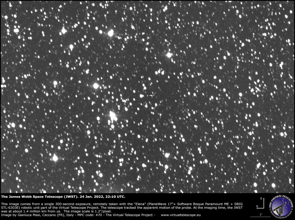
To mark the occasion, the Virtual Telescope Project (VTP) captured images of James Webb to give people a sense of what it looks like in orbit. Unfortunately, there’s not a lot to see there, other than a bright dot in the night sky. But like Carl Sagan’s famous “Pale Blue Dot” picture of Earth (taken by Voyager 1 on its way out of the Solar System), or Cassini’s “The Day Earth Smiled” image, there’s a tremendous amount of significance in that small point of light.
The James Webb Telescope imaged from Earth. – January 24th, 2022. Credit: TVTP 2.0
The image of the JWST (shown above) was taken on January 24th using Elena. This robotic telescope tracked the apparent motion of the JWST automatically and acquired a single 300-single unfiltered exposure that shows the telescope’s position (indicated by an arrow in the center). When it was imaged, the JWST had reached its final destination (L2), placing it at a distance of about 1.4 million km (869,920 mi) from Earth.
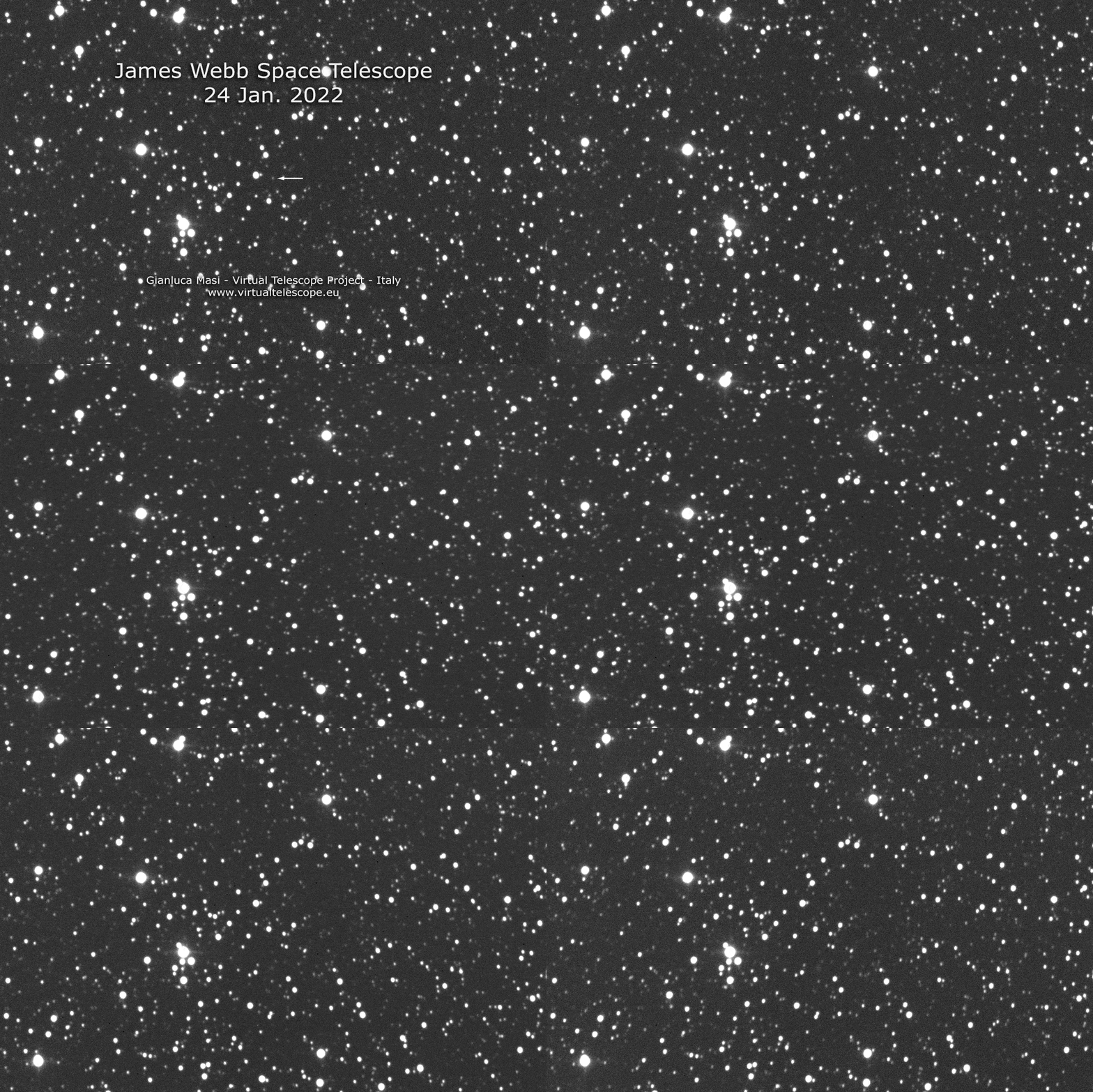
In addition to the above image, the VTP also created a short GIF animation (below) that shows the JWST’s apparent motion against the stars. While it may look like little more than a tiny dot against a background of brighter dots (and the darkness of space), these images tell a story of an ambitious mission that was decades in the making. Work began on the telescope in 1996, and it was initially hoped that the James Webb would be launched by 2007 and with a budget of $500 million.
Unfortunately, there were many delays and cost overruns due to a major redesign, issues with the sunshield, and the Ariane 5 rocket that would launch it. The COVID-19 pandemic also imposed delays, as did the fact that the James Webb is the most complex and advanced space telescope ever conceived. Time and again, the origami-like nature of the telescope (where it has to fold up to fit within a payload fairing) required extensive testing runs, and the slightest issues required retesting and safety checks.
By 2016, construction was finally finished, but an extensive testing program still had to be completed. By late 2021, the telescope testing finished up, and the James Webb was shipped to Kourou, French Guiana, for integration with the Ariane 5 rocket. When the launch finally happened on Christmas Day, it went off without a hitch. Thomas Zurbuchen, NASA’s associate administrator for science missions, commented, “It’s truly Christmas with all the presents and everything and we have a space mission!”
The James Webb Space Telescope in motion against the stars. January 24th, 2022. Credit: TVTP 2.0
By 2016, construction was finally finished, but an extensive testing program still had to be completed. By late 2021, the telescope testing finished up, and the James Webb was shipped to Kourou, French Guiana, for integration with the Ariane 5 rocket. When the launch finally happened on Christmas Day, it went off without a hitch. NASA’s associate administrator for science missions Thomas Zurbuchen, “It’s truly Christmas with all the presents and everything and we have a space mission.”
Now that the mission is at L2, the mission team is waiting for the telescope to reach operational temperature. This will be followed by the activation of the telescope’s instruments, final testing, and calibration. Barring any issues, NASA anticipates that the James Webb will begin collecting its first light by June 2022. As NASA Administrator Bill Nelson said:
“Webb, welcome home! Congratulations to the team for all of their hard work ensuring Webb’s safe arrival at L2 today. We’re one step closer to uncovering the mysteries of the universe. And I can’t wait to see Webb’s first new views of the universe this summer!”
Just 4,000 light-years from Earth is a strange, star-sized object. It’s been observed by radio telescopes, but astronomers aren’t sure what it is. They call it a long period transient.
Transients are objects in the sky that change over some period of time. Fast transients are things such as pulsars, which emit a bright flash over a period of seconds or milliseconds. Slow transients are objects such as supernovae, which grow to extreme brightness over days or months. This new object is transient three times an hour. About every 18 minutes, it becomes one of the brightest radio objects in the sky, with its flash lasting anywhere from half a second to nearly a minute. Its long period and extreme brightness are what makes it so unusual.
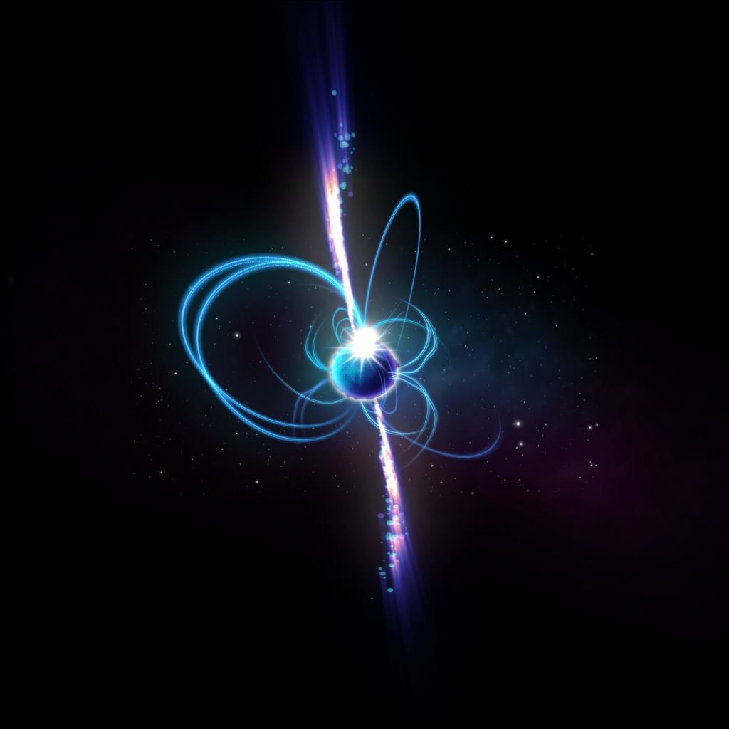
One idea is that the object is a hypothetical object known as an ultra-long period magnetar. Magnetars are neutron stars, the same as pulsars, but magnetars have much stronger magnetic fields. Most magnetars are thought to rotate as quickly as pulsars, but their strong magnetic fields could interact with surrounding ionized gas in a way that causes it to slow down significantly. This would turn it into a kind of slow rotating pulsar. The problem with this idea is that astronomers have thought ultra-long period magnetars wouldn’t be nearly so bright. Another idea is that the object is a strange type of white dwarf, but it isn’t clear how a white dwarf could become so radio bright.
An artist view of the object as a magnetar. Credit: ICRAR
Based on observations, we do know the object has an intense magnetic field. The radio light we see from the object is highly polarized. Charged particles emit highly polarized light when they interact with a strong magnetic field. We also know the transient can’t simply be a standard pulsar effect. Pulsars emit regular flashes because their rotation sweeps a beam of intense radio light across the sky. We see a radio flash every time the beam sweeps our way, similar to the flash of a lighthouse. This object would flash about every 18 minutes, but these flashes would only happen over the course of a few hours. The team saw the object shift between active and quiet periods during their observation runs. So some strange happenings are going on.
Of course, the most exciting idea is that the transient object is something we don’t expect. Perhaps a newly formed black hole, or a hypothetical quark star. With only one example, it’s difficult to narrow down the possibilities. So the team is searching for similar objects in order to solve the mystery they never expected to find.
Is this a closeup look at a tree stump, or an orbital view of an impact crater? At first glance, it might be hard to tell. But this image of a crater on Mars provides planetary scientists almost the same kind of climate history data about the Red Planet as tree rings provide to climate scientists here on Earth.
This picture was taken by the Colour and Stereo Surface Imaging (CaSSIS) camera onboard the ESA/Roscosmos ExoMars Trace Gas Orbiter (TGO), which arrived at Mars in 2016 and began its full science mission in 2018.
This unnamed crater is located in the vast northern plains of Acidalia Planitia. This plain is north of Valles Marineris, and the region contains the famous Cydonia region (where the “Face on Mars” butte is (it aoesn’t actually look like a face), and well as heavily cratered highland terrain.
So, why does this crater look so unusual? Scientist from the ExoMars mission say the interior of the crater is likely composed of ice-rich material, and the quasi-circular and polygonal patterns of fractures could be the result of seasonal changes in temperature that cause cycles of expansion and contraction of those materials, eventually leading to the development of fractures.
Along the crater rim on the left, possible gullies are also visible.
An unusual crater on Mars, as seen by the CaSSIS camera onboard the ESA/Roscosmos ExoMars Trace Gas Orbiter (TGO) on 13 June 2021 in the vast northern plains of Acidalia Planitia. Credit: ESA/Roscosmos/CaSSIS.
Any water-ice rich soil would have been laid down during an earlier time in Mars’ history when the inclination of the planet’s spin axis allowed such deposits to form at lower latitudes than it does today. Just like on Earth, Mars’ tilt gives rises to seasons, but unlike Earth its tilt has changed dramatically over long periods of time.
“Understanding the history of water on Mars and if this once allowed life to flourish is at the heart of ESA’s ExoMars missions,” say mission scientists. “The spacecraft is not only returning spectacular images, but also providing the best ever inventory of the planet’s atmospheric gases with a particular emphasis on geologically and biologically important gases, and mapping the planet’s surface for water-rich locations.”
This topographical map of Mars from the Mars Global Surveyor laser altimeter instrument shows the various regions on Mars.Acidalia Planitia can be see at the top near the center. Credit: MGS/MOLA.
The ExoMars orbiter will also provide data relay services for the second ExoMars mission which has the Russian built Kazachok lander that will bring the Rosalind Franklin rover to the surface of Mars. That mission is scheduled to launch in September of 2022. When it arrives on Mars in 2023, the rover will explore another region of Mars – not yet disclosed — thought once to have hosted an ancient ocean, and will search underground for signs of life.
Is Mars home to an underwater lake? Different researchers are reaching different conclusions. Some say remote sensing from the Mars Express orbiter shows liquid water in an underground lake at Mars’ south polar region. Other researchers say clays or minerals explain the data better.
Who’s right? Maybe none of them.
A new study says that volcanic rock can explain the Mars Express data and that it’s a more plausible explanation.
The Martian lake hypothesis dates back to 2018 when a team of researchers published a paper presenting data from the MARSIS (Mars Advanced Radar for Subsurface and Ionosphere Sounding) instrument on the ESA’s Mars Express orbiter. The data showed a highly-reflective surface under the South Polar Layered Deposits (SPLD). In that paper, the researchers concluded that water was responsible for the signal and the Mars lake hypothesis gathered steam.
Then other researchers published other papers giving different explanations for the signal, showing how clays and minerals might be responsible. Then MARSIS data showed more reflective areas which scientists interpreted as more subsurface lakes. Recently the authors responsible for the 2018 paper that started it all published a research letter re-affirming their original interpretation of the data and refuting research that reached different conclusions.
Now a group of scientists published a paper saying the other researchers have it wrong. They conclude that volcanic rock is responsible for the MARSIS signal.
The title of their paper is “The Basal Detectability of an Ice-Covered Mars by MARSIS.” The journal Geophysical Research Letters published the paper, and the lead author is Cyril Grima, a planetary scientist at the University of Texas Institute for Geophysics (UTIG).
The hypothesis that there’s water under the SPLD relies on a couple of facts. The water must be briny to resist freezing, and the temperature can’t be too low. Obviously, there’s a lot more detail than that involved. But that’s the essence of it. The temperature is critical because different materials display different permittivity at different temperatures. And scientists don’t know exactly what the temperature is under the SPLD.
This is a map of the SPLD thickness, based on MARSIS measurements and MOLA surface topography. Image Credit: Plaut et al. 2007.
But this paper sets some of those concerns aside.
“For water to be sustained this close to the surface, you need both a very salty environment and a strong, locally generated heat source, but that doesn’t match what we know of this region,” lead author Cyril Grima said in a press release.
Rather than clays, minerals, or brines, this new research suggests that a type of volcanic rock that’s relatively common on Mars is responsible for the MARSIS data. If some of that volcanic rock were buried under the ice in the SPLD, then it would appear bright like water when MARSIS observed it.
In the study, Grima and his co-authors used computer models to add a global sheet of ice onto the Martian surface. This simulated one-mile-thick ice sheet allowed the researchers to compare features all across Mars’ surface with those under the real ice at the south pole. The SPLD is about 10% impure, and the team duplicated that in their simulated ice.
The result?
A radar map of Mars as seen through a mile of ice. UT Austin planetary scientist, Cyril Grima, built a computer model to cover the Red Planet in ice and observed how it changed the radar data. This caused volcanic plains (seen in red) to reflect radar in a manner that resembled liquid water. The finding challenges a 2018 study that appeared to find liquid water under Mars’ south polar cap. Credit: Cyril Grima
The team found bright reflections like those under the SPLD scattered across different latitudes. Many of them matched up with known locations of volcanic rock. Overall they found that between 0.3% and 2.0% of Mars’ surface could produce the same MARSIS signal detected under the SPLD. The bright terrains the team detected in their study are “… gathered within volcanic constructs of diverse geologic epoch,” the paper says.
Not all of Mars’ known volcanic terrains produce the same signal. But some pronounced volcanic features like shield volcanoes produced strong reflections. “A broad region of strong reflections is identified East of the Uranius Tholus interpreted as a shield volcano resulting from effusive eruptions of low viscosity lavas during the Hesperian-Amazonian transition,” the authors write.
The study showed a strong connection between known volcanic areas and reflectivity. This image shows the Uranius Tholus shield volcano in yellow. The team found strong reflections to the east of the volcano. Image Credit: Wikimedia
There’s a fascinating scientific debate playing out right now over the potential water under the SPLD. These results won’t end that debate, but they play a role. “It draws attention that the brightest terrains across the planet would produce basal echoes with a radiometric character in the range of the brightest ones observed at the SPLD by Orosei et al. (2018) and under similar assumptions for the composition of the overlying ice.” (Note: Orosei et al. 2018 is the original study presenting evidence for liquid water under the SPLD.)
“This radiometric similarity (or continuity) is indicative of the likelihood for a non-wet generic material currently available at Mars to be responsible for the bright basal SPLD reflection,” the paper’s conclusion says. The non-wet material is an iron-rich volcanic rock that’s common on Earth, too.
What do scientists on the other side of this issue think?
Dr. David Stillman is a geophysicist at the Southwest Research Institute (SwRI.) He’s a co-author of papers in support of the liquid water hypothesis.
He told Universe Today that Grima et al. is a robust study. “The Grima paper is very good,” Dr. Stillman said. But he identifies some potential discrepancies if we can call them that, and points them out.
“His paper makes the assumption that surface MARSIS amplitudes can be compared even though they were processed onboard Mars Express when Mars’ magnetosphere was varying. The reflectivity data used by the Italian group (Orosei et al. 2018) was not processed onboard so that amplitudes could be compared when Mars’ magnetosphere was varying (another issue with assumptions).” Dr. Stillman is referring to assumptions about Mars that all scientists have to make when studying the planet. In particular, scientists must work with assumptions about the subsurface temperature under the SPLD. The temperature affects the reflectivity of different compounds, altering the MARSIS signal.
Grima and his co-authors used a figure to present some of their findings in their paper. It highlights four areas on the surface of Mars that show high reflectivity under the simulated ice sheet and shows how volcanic rock can account for the signal.
This figure from the study shows the relative basal echo strength of Mars if the surface was entirely covered by a 1.4-km dirty ice sheet (10% volume impurity rate). Bottom inserts display only positive values for better identifications relative to the regional landforms. Image Credit: Grima et al. 2022.
According to Grima et al., the fact that these four regions are spread across longitudes is a significant strength in their results. “Four insets in Figure 3 highlight some of those regions where a positive Pss/Ps signature is consistent across longitudes instead of just being confined locally along an orbit (an indicator of possible data glitch),” the paper says.
But Dr. Stillman said there’s another possibility for those signals.
“Additionally, if you look at Fig 3 of Grima’s paper you will see very high surface reflection in the northern plains of Mars that likely does not have massive lava flows, but are due to artifacts due to the onboard processing,” he said.
“All those arrows point to high reflectivity that is likely just artifacts as the majority of these are in what we think are sediments and could not have high dielectric values or reflectivity,” Stillman pointed out. “Solis Planum also has pretty random high values, does this mean the whole thing has a high reflectivity or just like 10% of it?”
This won’t be the end of the debate, but it does reveal how intricate the problem is.
This issue is important to many in the planetary science community. If you scan the internet you can see it gets lots of attention and lots of commentary from other researchers even though Martian polar scientists form a fairly small, tightly-knitted community.
The coloured dots in this image represent sites where the ESA’s Mars Express Orbiter spotted bright radar reflections at Mars’ south polar cap. Some researchers interpret the reflections as subsurface liquid water, but other researchers have different explanations. Credits: ESA/NASA/JPL-Caltech
Isaac Smith is a Mars geophysicist at York University who’s not involved in any of these studies. In a press release, Smith explained that the highly reflective signal could be explained by a type of clay dissolved in water. This phenomenon is present on Earth and could be on Mars, too.
Smith also points out that if Grima is right about the reflective signal, it’s not all bad when it comes to the larger issue of Martian water.
“I think the beauty of Grima’s finding is that while it knocks down the idea there might be liquid water under the planet’s south pole today, it also gives us really precise places to go look for evidence of ancient lakes and riverbeds and test hypotheses about the wider drying out of Mars’ climate over billions of years,” Smith said.
We’re in a position between competing hypotheses. But we’re not stuck. This is how science works.
“Science isn’t foolproof on the first try,” said Smith. “That’s especially true in planetary science where we’re looking at places no one’s ever visited and relying on instruments that sense everything remotely.”
Dr. Stillman seems to agree and points out that everyone is forced to make some assumptions when it comes to Mars.
“Honestly, I do not know which assumptions are correct because we are studying a planet so far away with very limited data,” he told Universe Today.
None of the papers published so far proves there’s water, and none prove there isn’t. Instead, we’re inching our way toward knowing for sure.
We need better data, which means we need another mission to Mars.
In the history of science and physics, several scholars, theories, and equations have become household names. In terms of scientists, notable examples include Pythagoras, Aristotle, Galileo, Newton, Planck, and Hawking. In terms of theories, there’s Archimede’s “Eureka,” Newton’s Apple (Universal Gravitation), and Schrodinger’s Cat (quantum mechanics). But the most famous and renowned is arguably Albert Einstein, Relativity, and the famous equation, E=mc2. In fact, Relativity may be the best-known scientific concept that few people truly understand.
For example, Einstein’s Theory of Relativity comes in two parts: the Special Theory of Relativity (SR and the General Theory of Relativity (GR). And the term “Relativity” itself goes back to Galileo Galilee and his explanation for why motion and velocity are relative to the observer. As you can probably tell, explaining how Einstein’s groundbreaking theory works require a deep dive into the history of physics, some advanced concepts, and how it all came together for one of the greatest minds of all time!
To break it down, Einstein proposed SR in 1905 to resolve experiments involving light with classical physics. Over the next ten years, Einstien would attempt to generalize the theory to explain how electromagnetism and classic mechanics could be resolved with gravity – which yielded GR. While Einstein’s insights would be confirmed within a few years, they continue to be tested and validated to this very day.
Prof. Albert Einstein delivering the 11th Josiah Willard Gibbs lecture at the meeting of the American Association for the Advancement of Science in on Dec. 28, 1934. Credit: AP Photo
As Einstein is credited with once saying, “If you can’t explain it to a six-year-old, you don’t understand it yourself.” But as noted already, doing that means getting into some history and advanced concepts – like universal gravitation, inertial reference frames, mass-energy equivalence, spacetime, etc. But with a little patience and dedication, the theory of Relativity is something that anyone is capable of understanding.
Galileo and Newton
The story of Relativity goes back to the 17th century and the work of famed Italian astronomer and polymath Galileo Galilee. In 1632, Galileo published Dialogue Concerning the Two Chief World Systems, which many consider to be his magnum opus. In this work, Galileo explained in simple terms how the Heliocentric Model of the Universe (as described by Copernicus) resolved issues that the Geocentric Model could not explain. Among other things, Galileo explained why the Earth’s motion was not obvious to people on its surface.
In keeping with his ability to convey complex ideas with simple and erudite logic, Galileo illustrated how this was possible using the metaphor of a ship at sea. In short, Galileo said that if a person standing on the deck were to drop a ball of wax into a vase of water, they would see the ball descend directly down to the bottom. This would apply regardless of whether the ship was in motion or not. The reason, he stated, is because the ball and everything aboard the ship is part of the ship’s inertial reference frame – i.e., it moves with it.
The same, he argued, holds for a person standing on the surface of Earth as it moves:
“Now these things take place in motion which is not natural, and in materials with which we can experiment also in a state of rest or moving in the opposite direction, yet we can discover no difference in the appearances, and it seems that our senses are deceived.
“Then what can we be expected to detect as to the earth, which, whether it is in motion or at rest, has always been in the same state? And when is it that we are supposed to test by experiment whether there is any difference to be discovered among these events of local motion in their different states of motion and of rest, if the earth remains forever in one or the other of these two states?”
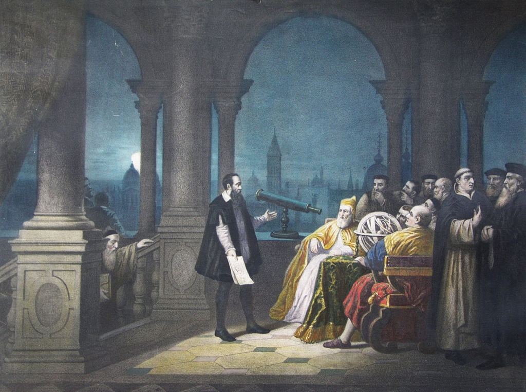
Galileo Galilei displaying his telescope to Leonardo Donato. Credit: Wikimedia Commons
However, to an observer on the shore, Galileo claimed that things would look quite different. If the person standing on the ship’s deck dropped the ball over the side, it would appear to them that it still fell straight down. But to the observer on the shore, it would look like it was following a parabolic path. To them, the ball’s motion would visibly be the result of motion imparted by the moving ship with the Earth’s gravitational pull. In short, the motion and velocity would be relative to the observer.
This came to be known as Galilean Relativity (or Galilean Invariance), which came down to a single postulate: “[A]ny two observers moving at constant speed and direction with respect to one another will obtain the same results for all mechanical experiments.” In other words, the physical mechanics of a system are the same in all reference frames, provided the motion and velocity of the observers remain constant. However, if either of these parameters changes, then the mechanics will change (more on that later).
The explanation would become a key argument used in defense of the Heliocentric Model. For Earth-based observers, the motions of the planets, the Sun, the Moon, and the stars were all relative to the observer (us). But when one cataloged the motions (and the relative size) of these objects in the night sky over time, they would see how these observations could only be explained by the motion of the Earth around the Sun (as well as the rotation of Earth itself) at a constant velocity.
By 1687, Sir Isaac Newton would revolutionize our understanding of physics with his magnum opus, Philosophiæ Naturalis Principia Mathematica. In this tome, Newton synthesized Galileo’s theories on motion with his research into gravitation, which was summarized with his Three Laws of Motion. These included:
A body continues in its state of rest, or in uniform motion in a straight line, unless acted upon by a force.
A body acted upon by a force moves in such a manner that the time rate of change of momentum equals the force.
If two bodies exert forces on each other, these forces are equal in magnitude and opposite in direction.
These three laws describe three physical constants that remain central to modern physics: Intertia, which states that bodies will remain in a state of motion unless an external force speeds them up or slows them down; Force, which can be summarized mathematically as the mass of an object multiplied by its acceleration (F=ma); and Action-Reaction, which establishes when an object exerts a force on another object, the second object exerts an equal and opposite on the first.
This laid the groundwork for Newton’s Universal Gravitation, which states that all point sources with mass attract each other through gravitational force; and the Inverse Square Law, which states that this force is directly dependent on the masses of both objects and inversely proportional to the square of the distance between their centers. In short, Newton argued that the same force that caused the apple to fall from a tree (Newton’s Apple) causes the planets to orbit the Sun, the Moon to orbit Earth, and all other orbital mechanics in the Solar System.
A consequence of Newton’s Universality was that scientists would henceforth see space and time as reference frames that were fixed and separate. Basically, an object’s position and motion could be described in terms of three dimensions in space – length, height, and depth (or the x, y, z axes) – and one dimension in time. This framework for understanding the Universe would become canon for the next two hundred years. Newton’s theories were so influential that the terms Classical Physics and Newtonian Physics (or Mechanics) would be used interchangeably.
By the mid-to-late 19th century, new discoveries in the fields of astronomy, electromagnetism, and particle theory would knock these conventions on their ear. What had previously seemed like an orderly Universe consisting of space and time, matter and energy, and universal reference frames would be replaced by relativistic effects, time dilation, and “spooky action at a distance.”
Electromagnetism
By the mid-19th century, scientists had made multiple breakthroughs in the study of optics (light and colors) and electromagnetic (EM) phenomena. This led to the realization that light is a form of EM radiation and that its properties (how it behaves like a wave) were similar to the propagation of electrical current. Moreover, experiments performed by this time yielded highly-accurate estimates in the speed of light – 299,792,458 m/s (1.079 billion km/h; 670.6 million mph).
In addition, the theoretical work of James Clerk Maxwell and Hendrik Lorentz established that electric and magnetic forces behaved as fields that exert force on point charges. These were summarized in Maxwell’s Equations (1861-62) and the Lorentz Force Law (1895), which describe how electric and magnetic fields are generated by charges, currents, and changes of the fields. Together, these principles form the basis of classical electromagnetism, optics, and electric circuits.
These experiments also yielded highly-accurate estimates for the speed of light – which is currently clocked at 299,792,458 m/s (1.079 billion km/h; 670.6 million mph). Unfortunately, these experiments also presented theoretical problems as far as Classical Physics was concerned. In all cases, the measured speed of light was constant, regardless of whether the source was moving relative to the observer or not. This contradicted a basic tenet of Classical Mechanics and Galilean Relativity.
For example, Earth’s rotation on its axis essentially means that it is rotating towards the Sun. This means that when the Sun is in the east, the light reaching an observer would be approaching and therefore have a greater measured velocity than light observed from any other direction. However, experiments involving optics and the refraction of light, like those performed by Augustin Fresnel in 1818, showed no measurable change in the speed of light.
The Mysterious “Aether”
As a result, scientists began postulating by the early 19th century that space must be filled with some invisible “aether.” This medium, they argued, allowed light to propagate through space but also meant that light was dragged along by it – leading to a change in its velocity. This was exemplified by Fresnel’s partial aether-drag hypothesis, where he stated that the motion of the Earth does not have any influence on how light refracts because “the ether is partially carried along by the earth and light waves inside the optical medium are partially dragged along with the ether.”
This is similar to how sound travels in air or water or ripples propagate across the surface of a pond. Alas, the experiments conducted throughout the 19th century continually indicated that the speed of light was constant. To resolve these theoretical issues with the experimental results, scientists needed to measure the effects of this aether to determine its properties. This required that scientists show that the measured speed of the light was a simple sum of its speed through the medium, plus the speed of the medium.
Hippolyte Fizeau attempted to prove this with his “water tube experiment” (or Fizeau experiment), which he conducted in 1851. After measuring the speed of light in moving water through tubes, Fizeau’s results indicated that light was being dragged along by the medium – the water. This appeared to confirm earlier experimental results, such as those conducted by Augustin Fresnel and Sir George Strokes. However, the magnitude of the effect that Fizeau observed was far lower than expected.
Another famous example was the Michelson-Morley Experiment (1887) conducted by American physicists Albert A. Michelson and Edward W. Morley. Using a chamber and a series of mirrors, they attempted to measure the speed of light from different angles – a horizontal one corresponding to Earth’s rotation towards the Sun and a perpendicular one. If such an “aether” existed, then the Earth’s movement through it (and towards the Sun) would result in a noticeable difference with the horizontal beam.
Once again, the experiment yielded negative results since there was no observable difference between the measured speeds of the light beams. At this point in the game, Einstein would come along and offer a brilliant insight, analysis, and synthesis of the theoretical and experimental data. This occurred in 1905 when Einstein first revealed what would be known as his Theory of Special Relativity (SR).
Enter Einstein
In 1905, during his “annus mirabilis” (miracle year), Einstein published his dissertation, as well as four groundbreaking papers that would bring him to the notice of the international scientific community. One of them was “On the Electrodynamics of Moving Bodies,” where Einstein proposed what would come to be known as his Theory of Special Relativity (SR). This theory resolved Maxwell’s equations and the Lorentz force law with Newton’s Laws of Motion and came down to two postulates:
The laws of physics are identical in all non-accelerated inertial reference frames
The speed of light in a vacuum is constant, regardless of the motion of the observer or light source
A key aspect of Einstein’s breakthrough was Lorentz Transformations, which the elder physicist derived when examining the experiments concerning the behavior of light. To explain why light did not conform to Relativity, Lorentz theorized that things become distorted (compacted) along the path of travel in an accelerated inertial reference frame. As Einstein theorized, objects approaching the speed of light (c) will observe no change in c coming from external sources, but they will notice time is moving slower for them than the
Like his predecessor, Galileo, Einstein related the mechanics of this concept using a metaphor, a slightly updated one at that. According to Einstein, a person traveling on a train will notice the same relativistic effects Galileo mentioned, where a ball will fall straight to the floor. To an observer beside the tracks, the same boll dropped over the side of the train would appear to fall along a parabolic path. Now substitute the ball with a series of mirrors.
The person riding the train holds one in their hand while another is directly beneath it on the floor. To the person holding the mirror, a beam of light would appear to be bouncing up and down repeatedly. Now imagine another mirror is located on the wall at the head of the car. If the person reoriented the mirror in their hand to face it, a beam of light would appear as if it were bouncing back and forth across the train car. In all cases, the light would appear to be traveling at a constant speed (c).
But to the person standing beside the tracks, the light would appear to be zig-zagging along in the first scenario, trying to catch up with the moving mirrors. In the second scenario, it would appear as if the light were moving slower as it went from the handheld mirror to the one in the front of the car. Alas, if they could time it, they too would record a constant speed of c. Instinctively, this would make little sense to the two observers until they consulted their watches.
For the person riding in the train cart, time would have moved (infinitesimally) slower. The difference would be immeasurable, but if the moving reference frame were something like a spacecraft capable of traveling at a fraction of the speed of light, the difference would be impossible to miss. Essentially, the person in the moving reference frame has experienced time at a slower rate, an effect known as “time dilation.” As objects get closer and closer to the speed of light, this effect increases.
However, Einstein and his contemporaries still held to the Conservation of Energy Law first proposed and tested by Émilie du Châtelet in the 18th century. This law states that the total energy of an isolated system remains constant and is conserved over time. Applying this same reasoning to objects approaching the speed of light, Einstein’s derived the equation E=mc2, where E is the total amount of energy in a system, m is the system’s mass, and c is the system’s acceleration towards the speed of light.
According to this law, objects accelerating towards the speed will experience an increase in their inertial mass. This means that more energy is required to maintain the object’s acceleration over time and that the speed of light is absolute. Not only would an object require an infinite amount of energy to achieve the speed of light, but its mass would also become infinite in the process. Another startling consequence was how mass and energy are interchangeable in this equation.
If mass and energy are switched around in the equation, the outcome remains the same. This came to be known as the principle of Mass-Energy Equivalence, which states that energy and mass are essentially two sides of the same coin. Another consequence of SR is how it interprets space and time as two expressions of the same reality. Per Newtonian Physics, scientists viewed the geometry of the Universe in terms of three dimensions – height, length, and width (or an x, y, and z axes) – and one dimension of time.
In other words, Newtonian Physics viewed space and time as separate and fixed. But by showing how time was relative to the observer in an accelerated reference frame, Einstein’s presented a four-dimensional geometry consisting of three dimensions of space and one dimension of time – aka. Spacetime! Almost immediately, scientists began adopting Einstein’s SR because of the way it resolved electromagnetism with Newton’s theories of motion and for how it did away with the need for an “aether.”
General Relativity
Between 1905 and 1915, Einstein sought to generalize SR by extending it to account for gravity. This was largely due to theoretical problems arising from Newton’s theory of Universal Gravitation. Previously, astronomers found that Newton’s equations could account for the orbits of most of the then-known Solar bodies. However, Mercury’s orbit presented a long-term peculiarity that Newton’s equations couldn’t account for. In addition to having a highly-eccentric orbit, Mercury’s perihelion also moves around the Sun over time.
This is known as a “precession of perihelion,” where the farthest point in a planet’s orbit moves around the parent body over time. There was the way Newton’s theories interpreted gravity as an attraction between point sources with mass. But if this were true, then the force of attraction would be something that occurred instantaneously between objects, even if it was particularly weak over long distances. But as Einstein demonstrated with SR, information is not communicated instantaneously across spacetime.
There were also several outstanding issues regarding how SR applied to the Universe at large. The first issue was the idea of instantaneous communication. As Einstein previously demonstrated with SR, information is not communicated instantly across spacetime but is limited to the speed of light. A supernova that takes place 1 billion light-years away will appear to be presently exploding in the night sky to us but took place 1 billion years ago.
In keeping with the laws of electromagnetism, Einstein ventured that gravity acted as a field rather than an instantaneous pull. The greater the mass, the more powerful the field within which objects would be attracted to each other. Another important issue was acceleration, which Einstein illustrated using another clever (and updated) metaphor: a passenger on an elevator. If someone were to cut the cable, the elevator would begin to fall at a rate of 9.8 m/s2 (Earth-normal gravity, or 1 g) towards the center of the Earth.
The passenger would experience the sensation of weightlessness (freefall) right up until the point where the elevator crashed! The same holds for any object experiencing acceleration, be they boats, planes, trains, automobiles, or spacecraft. At a constant velocity, people traveling within an inertial reference frame (in the absence of external reference points) would not be aware that they were even moving. In fact, a passenger or crew in space would feel weightless if the spacecraft were at rest or moving at a constant velocity.
But if the reference frame accelerated, anyone inside would be thrust in the opposite direction of travel. If the acceleration were equal to 9.8 m/s2, the crew would experience the sensation of Earth-normal gravity. If the spacecraft were oriented with its vertical axis pointed in the direction of travel, the acceleration would keep the crew’s feet firmly planted on the floor. The same principle applies to pinwheel stations or rotating cylinders in space, where the rotational velocity generates a centripetal force that causes objects to be pulled outwards.
For people aboard the station, this force creates the sensation of gravity. Depending on the radius and velocity of the station, the “artificial gravity” can be equal to Earth-normal gravity. Since the late 20th century, many noted scientists have proposed that such facilities could be the key to exploring and settling the Solar System – including Konstantin Tsiolkovsy, Werner von Braun, and Gerard K. O’Neill (where the O’Neill Cylinder gets its name). The bottom line is that acceleration is indistinguishable from gravity in an inertial reference frame.
Last, but not least, there was the issue of time dilation, as raised by SR and Lorentz Transformations. If acceleration causes time dilation, then this means that gravity itself has an effect on spacetime. From this, Einstein’s General Relativity (GR) was born! Instead of gravity being a force of attraction between point masses, said Einstein, gravity itself is a consequence of the curvature of spacetime, which is altered by the presence of a massive object. Ergo, when objects orbit one another, they are not being “pulled,” but tracing the curvature of that spacetime.
In November 1915, Einstein presented his Field Equations to the Prussian Academy of Science in Berlin, Germany. These equations specify how the four-dimensional geometry of spacetime is influenced by gravitational fields (mass) and radiation (electromagnetic forces). In the words of John Wheeler, “spacetime tells matter how to move; matter tells spacetime how to curve.” From all of this, Einstein’s General Theory of Relativity (GR) was officially born and would quickly become foundational to our modern understanding of physics.
Much like SR, Einstein’s generalized theory of Relativity would have several theoretical consequences. For starters, if what Einstein was saying was true, it meant that gravitational fields and the resulting curvature of spacetime would affect everything, including light! This prediction presented astrophysicists with the means to test GR, and the first opportunity came in 1919. At this time, Frank Dyson, Arthur Eddington, and a team of astrophysicists conducted an experiment during a solar eclipse (the Eddington Experiment).
Eddington Experiment
In the century since Einstein’s formalized his theory, SR and GR have been repeatedly tested and validated. Some of these tests involved small-scale experiments, while others were conducted under the most extreme conditions. In the case of the Eddington Experiment (or Expedition), the test consisted of observations made during a solar eclipse from two equatorial observatories – one located on the northeast coast of Brazil, the other on the island of Sao Tome and Principe off the coast of West Africa.
Specifically, the expedition team was looking for stars passing behind the Sun during the eclipse. If Einstein’s theory were correct, the light coming from these stars would trace the spacetime curvature caused by the Sun’s gravity. To the observers, this effect would make it look like the stars themselves were next to the Sun. With the Sun’s radiance effectively blocked by a total eclipse by the Moon, the light would be visible to their expeditions’ instruments.
Not only did the teams at both observatories see these stars, but their positions in the night sky were precisely where Einstein’s Field Equations predicted they would be. The story was immediately picked up by newspapers worldwide and posted on their front pages, making Einstein and General Relativity an overnight sensation! However, this was one of many tests and predictions that ultimately proved Einstein’s theories to be correct.
In time, GR would be incorporated into all areas of modern physics, ranging from electromagnetism and astrophysics to particle physics and the then-emerging field of quantum mechanics. Interestingly, some of the theories that would arise from Einstein’s breakthrough would not sit well with the astrophysicist. In fact, he would consider some of them (like cosmic expansion and quantum theory) to be downright heretical (and “spooky”)!
Cosmic Expansion
For example, in 1917, Einstein attempted to use GR to create a model of the structure of the Universe. To his dismay, he found that on the cosmic scale, his Field Equations predicted that the Universe was either in a state of expansion or a state of contraction. In order to prevent galaxy clusters and the large-scale structure of the Universe from collapsing in on itself, something needed to be counteracting gravity on the largest of scales. Since he preferred the idea of a constant and unchanging Universe (a common view at the time), Einstein introduced a new concept to GR.
This was known as the Cosmological Constant, represented by the mathematical character Lambda in his Field Equations. This force, he ventured, was responsible for “holding back gravity” and ensuring that the matter-energy density of the cosmos remained the same over time. By doing this, Einstein found himself caught up in the debate between proponents of the Steady State Hypothesis and the Big Bang Theory of cosmology (which would eventually be resolved in favor of the Big Bang model).
Einstein’s new theory would also attract challenges from some of his peers, who viewed it as an unstable fix to the problems presented by GR. In 1922, Russian physicist Alexander Friedmann mathematically showed how Einstein’s Field Equations were consistent with a dynamic Universe (The Friedmann Equation). This was followed by Belgian astrophysicist Georges Lemaître in 1927, who demonstrated that GR and an expanding Universe were consistent with astronomical observations, particularly those of American astronomer Edwin Hubble.
In 1931, Einstein visited Hubble at the Mount Wilson Observatory, where he witnessed how galaxies were receding from the Milky Way. In response to what Hubble presented him, Einstein formally announced that he was dropping the Cosmological Constant from his theories, claiming that it was the “biggest blunder of my career.” Meanwhile, astrophysicists would continue to measure the rate at which the cosmos was expanding, which would come to be known as Hubble’s Law (aka. the Hubble-Lemaitre Law). However, observations made throughout the 1990s (particularly with the Hubble Space Telescope) showed that the rate of cosmic expansion increased with time!
This led astrophysicists to theorize that there was a mysterious force counteracting gravity. But rather than preventing the Universe from collapsing on itself, this force was actively driving it apart. Today, we know this force as Dark Energy. Along with Dark Matter, it is a key ingredient to the most widely accepted cosmological model – the Lambda Cold Dark Matter (LCDM) model.
Black Holes, Lensing, and Waves
In 1915, just a few months after Einstein unveiled GR, German physicist and astronomer Karl Schwarzschild found a solution to Einstein’s Field Equations that predicted the existence of black holes. According to this solution, the mass of a sphere can become so compressed that the escape velocity from the surface would be equal to the speed of light. This is now called the Schwarzschild Radius, which describes the minimum dimensions a spherical mass must collapse to form a black hole.
In 1924, Eddington observed how Einstein’s theory allowed astronomers to rule out the existence of visible stars with overly large densities. According to Eddington, such dense bodies would “produce so much curvature of the spacetime metric that space would close up around the star, leaving us outside (i.e., nowhere).”
In 1931, Indian-American astrophysicist Subrahmanyan Chandrasekhar offered a resolution to SR by calculating how a sufficient mass of electron-degenerate matter (in a non-rotating body) would collapse in on itself. This came to be known as the Chandrasekhar Limit. When combined with Schwarzschild’s calculation, astrophysicists now had estimates on the mass and radius limits of black holes.
In 1939, Robert Oppenheimer and other scientists concurred with Chandrasekhar’s analysis, claiming that neutron stars above a prescribed limit would collapse into black holes. They also defined the outer boundary of the Schwarzschild radius as the edge of a singularity, within which time would stop. To external observers, a black hole would be perceived as a star frozen in time at the instant of collapse, but an infalling observer would have an entirely different experience.
Another effect predicted by GR is how gravitational fields can bend and focus light coming from more distant sources. This is known as Gravitational Lensing, where a particularly massive object acts as a “Lens” to amplify light forces beyond (or behind) it. This method has also been used to test Einstein’s GR under extreme conditions, such as observations of Sagittarius A*, the supermassive black hole (SMBH) at the center of the Milky Way. A modified version of this technique, Gravitational Microlensing, also detects exoplanets around distant stars.
Yet another prediction that emerged from GR is the rippling effect that gravitational forces can have on spacetime. This occurs when two particularly massive objects (neutron stars, black holes, or SMBHs) merge and release a tremendous amount of energy in the form of Gravitational Waves. The first confirmed detection of these waves was made by the Laser Interferometer Gravitational-Wave Observatory (LIGO) in 2016, roughly a century after Einstein first predicted them.
Einstein’s Theory of Relativity would also have a profound influence in the emerging field of Quantum Mechanics. The discoveries he would help make here were another source of consternation for him. Among them, the principle of quantum entanglement, which he would characterize as “spooky action at a distance,” and that the Universe was characterized by the semi-chaotic nature of Schrodinger’s Equation of quantum wave function and Heisenberg’s Uncertainty Principle.
Even though Einstein would resist some of the breakthroughs he helped inspire, the role he played in revolutionizing modern physics cannot be denied. Of all the contributions he made, however, none begin to approach the significance (or consequence) of Relativity. Over a century after he finalized his generalized theory, advanced experiments continue to demonstrate just how correct he was. Little wonder why it remains part of the foundation upon which modern physics, quantum physics, astrophysics, and cosmology rest.